PROB_L3

Independent events

We say two events are independent if $P(A\cap B)=P(A)P(B)$.
Events $A_1,\dots ,A_n$ are said to be independent if $P(A_1\cap A_2\cap \cdots \cap A_n)=P(A_1)P(A_2)\dots P(A_n)$ and any subcollection of $\{A_i\}$ containing at least two but fewer than $n$ events to be mutually independent.

Note that if $A_1,\dots ,A_n$ are pairwise independent, they need not be independent as a collection. For example, let $\Omega =\{a,b,c,d\}$ and let the probability function assign a probability of $\frac{1}{4}$ for each element in $\Omega$. Consider the events $A_1=\{b,c\}$, $A_2=\{b,d\}$, and $A_3=\{c,d\}$. $P(A_i)=\frac{1}{2}$, $P(A_i\cap A_j)=\frac{1}{4}$. Thus, the $A_i$s are pairwise independent. But, $P(A\cap B\cap C)=0$.

The notion of independence is frequently used to construct probability spaces corresponding to repetitions of the same experiment, where the outcome of each iteration of the experiment is not influenced by the results of the other iterations. Let $S_i=({\Omega }_i,P_i)$ be a discrete or finite probability space modeling the $i$th iteration of the experiment. The probability space for $n$ iterations of the experiment can be constructed like so: $S=({\Omega }_1\times {\Omega }_2\times \cdots \times {\Omega }_n,P)$, where $P$ is defined on the elementary events like so: $P(\{({\omega }_1,{\omega }_2,\dots ,{\omega }_n)\})={\prod }_{i=1}^n{P}_i({\omega }_i)$ (it is easy to verify that this definition satisfies the properties of a probability measure). Note that the event $C_i\subset {\Omega }_i$ occurring in the $i$th iteration would correspond to the event ${\Omega }_1\times \cdots \times C_i\times \cdots \times {\Omega }_n$ in the new probability space. As we would expect, this construction makes events that belong entirely to different iterations independent.

For example, let the experiment we wish to repeat be a coin toss. The probability space modeling a single coin toss is $\left(\{0,1\},\left\{(\{\},0),\left(\{0\},1-p\right),\left(\{1\},p\right),(\{0,1\},1)\right\}\right)$. The probability space $S$ modeling $n$ iterations of the experiment would have a sample space of $n$-tuples consisting of $0$s and $1$s. The probability of an elementary event would be computed like so:

$$P((0,1,1,0,1))=(1-p)(p)(p)(1-p)(p).$$

Going a little further, it is evident that all elementary events which produce the same total number of $1$s have the same probability. Let’s associate with every elementary event in $S$ a number $X$ which counts the number of $1$s that appear in the event. $X$ is what is called a discrete random variable. One can say that the probability of getting $k$ $1$s is

$$P(X=k)=\left(\genfrac{}{}{0ex}{}{n}{k}\right)p^k(1-p{)}^{n-k}.$$

---

Discrete random variables

Definition 1(Definition).

A discrete real valued random variable $X$ on a probability space $(\Omega ,\mathcal{F},P)$ is a function $X:\Omega \to S\subset \mathbb{R}$, $|S|\le {\aleph }_0$ such that $\{\omega |X(\omega )=x\}\in \mathcal{F}$ for all $x\in S$.

Important

All random variables/vectors we will deal with before the midsem are going to be discrete ones.

$\{\omega |X(\omega )=x\}$ is usually shortened to $(X=x)$. In the previous example, $(X=3)$ would be the event corresponding to getting $3$ ones.

Note that if $X$ is a random variable on $(\Omega ,\mathcal{F},P)$ and $f:\mathbb{R}\to \mathbb{R}$ is any function, then $f\circ X$ is also a random variable, since $(f\circ X=c)={\bigcup }_{x\in f^{-1}(c)}(X=x)$.

Discrete density functions

Definition 2(Definition).

The real valued function $f:\mathbb{R}\to [0,1]$ defined by $f(x)=P(X=x)$ is called the discrete density function or discrete mass function of $X$. A number $x$ is called a possible value of $X$ if $f(x)>0$.

Properties of the probability mass function that should be obvious:

• $f(x)\ge 0$ for all $x\in \mathbb{R}$, and $f(x)>0$ for at most countably many $x\in \mathbb{R}$.
• ${\sum }_{x\in \mathbb{R}}f(x)=1$.

Also, for any function $f:\mathbb{R}\to [0,1]$ satisfying the above properties, there exists a probability space and a random variable $X$ with mass function $f$ (take the trivial example to show its existence). This result assures us that statements like “Let $X$ be a random variable with discrete density $f$” always make sense, even if we do not specify directly a probability space upon which $X$ is defined.

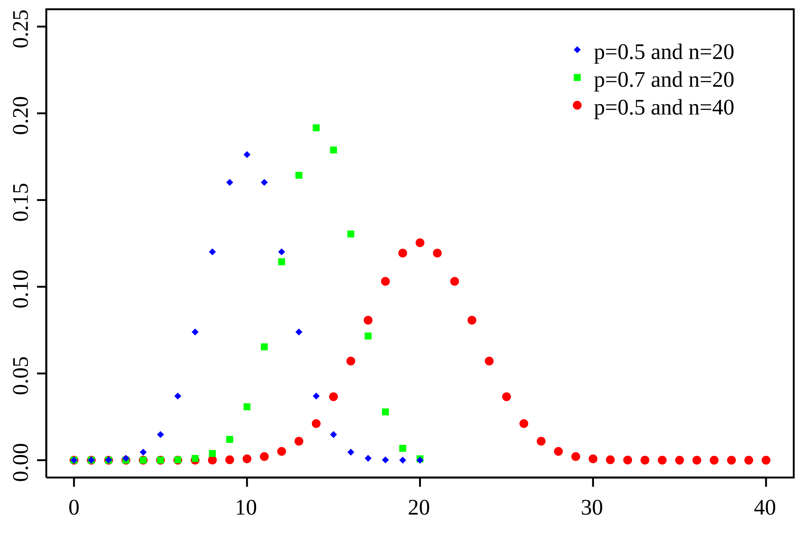
Binomial distribution

Consider $n$ independent repetitions of a simple success-failure experiment, like the coin tossing one discussed above. Let $S_n$ denote the number of successes in $n$ trials. Then, $S_n$ is a random variable that can only assume the values $0,1,\dots ,n$. The probability density for such an experiment is called the binomial density.

$$f(x)=\{\begin{array}{ll}\left(\genfrac{}{}{0ex}{}{n}{x}\right)p^x(1-p{)}^{n-x}& x\in \{0,1,\dots ,n\}\\ 0& \text{otherwise.}\end{array}$$

The outcome of performing $n$ Bernoulli trials with fixed parameter $p$ can be given by the random vector $\mathbf{X}=(X_1,X_2,\dots ,X_n)$, with $X_i=1$ and $X_i=0$ signaling success and failure in the $i$th trial respectively. We know that the random variable $S_n=X_1+X_2+\cdots +X_n$ is binomially distributed with parameters $n$ and $p$, as shown above. Turning this around, we can say that any random variable $Y$ that is binomially distributed with these same parameters can be thought of as the sum of $n$ independent Bernoulli random variables $X_1,\dots ,X_n$ each having parameter $p$.

The distribution function

What follows is valid for all probability spaces.

Definition 3(Definition).

If $X$ is a random variable on $\Omega$, define its distribution function by $F(x)=P(X\le x)=P(X\in (-\infty ,x])$.

Theorem 4(Proposition).

• $F$ is non decreasing.
• ${\lim }_{x\to \infty }F(x)=1$
• ${\lim }_{x\to -\infty }F(x)=0$
• ${\lim }_{x\to x_0^{+}}F(x)=F(x_0)$ for all $x$ (right continuity).

The fourth point is shown by considering any monotone decreasing sequence $({ϵ}_n)$ converging to $0$, and observing that

$$\begin{array}{rl}F(x_0)& =P(X\le x_0)\\ & =P((-\infty ,x_0])\\ & =\underset{n\to \infty }{\lim }P((-\infty ,x_0+{ϵ}_n])\\ & =\underset{n\to \infty }{\lim }F(x_0+{ϵ}_n),\end{array}$$

where these properties have been used. A closely related result is $F(x_0-)=P(X<x_0)$:

$$\begin{array}{rl}P(X<x)& =\underset{n\to \infty }{\lim }P(X\le x-{ϵ}_n)\\ & =\underset{n\to \infty }{\lim }F(x_0-{ϵ}_n).\end{array}$$

It follows that $F(x+)-F(x-)=P(X=x)$. This will be important when we discuss continuous random variables.

Also, any function satisfying the four properties in the proposition above is called a distribution function.