LEC ANA1 25

Taylor’s theorem

Let $f:[a,b]\to \mathbb{R}$ be twice differentiable. Fix $x\in [a,b]$. Consider the simplest approximation of $f$ that can be made: a constant function.

$$f(x+h)=\underset{E_0(h)}{\underbrace{f(x)}}+r_0(h)$$

Here, $E_0(h)$ is a constant polynomial approximation, and $r_0(h)$ is the error. Note that ${\lim }_{h\to 0}{r}_0(h)=0$. Now, we can try to refine our approximation by siphoning information from the error function. Consider the limit

$$\begin{array}{r}\underset{h\to 0}{\lim }\frac{r_0(h)}{h}=\underset{h\to 0}{\lim }\frac{f(x+h)-f(x)}{h}=f^{\prime }(x).\end{array}$$

Let

$$r_1(h)\equiv \frac{r_0(h)}{h}-f^{\prime }(x).$$

Clearly, ${\lim }_{h\to 0}{r}_1(h)=0$. Plugging in the value of $r_0(h)$ in terms of $r_1(h)$ in the zero degree approximation gives the first degree approximation $E_1(h)$ at $x$.

$$f(x+h)=\underset{E_1(h)}{\underbrace{f(x)+f^{\prime }(x)h}}+r_1(h)h,$$

How would you obtain a second degree approximation? Once more, consider the limit

$$\begin{array}{rl}\underset{h\to 0}{\lim }\frac{r_1(h)}{h}& =\underset{h\to 0}{\lim }\frac{f(x+h)-f(x)-f^{\prime }(x)h}{h^2}\\ & =\underset{h\to 0}{\lim }\frac{f^{\prime }(x+h)-f^{\prime }(x)}{2h}=\frac{f^{\prime \prime }(x)}{2}\end{array}$$

and let

$$r_2(h)\equiv \frac{r_1(h)}{h}-\frac{f^{\prime \prime }(x)}{2}.$$

Again, ${\lim }_{h\to 0}{r}_2(h)=0$. Plugging in the value of $r_1(h)$ in terms of $r_2(h)$ in the first degree approximation yields:

$$f(x+h)=\underset{E_2(h)}{\underbrace{f(x)+f^{\prime }(x)h+\frac{f^{\prime \prime }(x)}{2}{h}^2}}+r_2(h)h^2.$$

where ${\lim }_{h\to 0}{r}_2(h)=0$.

$E_n$ is called the $n$th Taylor polynomial at $x$.

Theorem 147.1(Pugh (2015) 3.12).

Assume that $f:(a,b)\to \mathbb{R}$ is $r$th order differentiable at $x$. Then

1. $E_r$ approximates $f$ to order $r$ at $x$ in the sense that the Taylor remainder $R(h)=f(x+h)-E_r(h)$ is $r$th order flat at $h=0$; that is, $R(h)/h^r\to 0$ as $h\to 0$.
2. $E_r$ is the only polynomial of degree $⩽r$ with this approximation property.
3. If, in addition, $f$ is $(r+1)$th order differentiable on $(a,b)$ then for some $\theta \in (x,x+h)$ we have

$$R(h)=\frac{f^{(r+1)}(\theta )}{(r+1)!}{h}^{r+1}.$$

Proof.

$(1)$ The first $r$ derivatives of $R(h)$ exist and equal $0$ at $h=0$. If $h>0$ then repeated applications of the Mean Value Theorem give

$$\begin{array}{rl}R(h)& =R(h)-R(0)=R^{\prime }({\theta }_1)h=(R^{\prime }({\theta }_1)-R^{\prime }(0))h=R^{\prime \prime }({\theta }_2){\theta }_{1}h\\ & =\cdots =R^{(r-1)}({\theta }_{r-1}){\theta }_{r-2}\dots {\theta }_{1}h\end{array}$$

where $0<{\theta }_{r-1}<\cdots <{\theta }_1<h$. Thus,

$$\left|\frac{R(h)}{h^r}\right|=\left|\frac{R^{(r-1)}({\theta }_{r-1}){\theta }_{r-2}\dots {\theta }_{1}h}{h^r}\right|⩽\left|\frac{R^{(r-1)}({\theta }_{r-1})}{{\theta }_{r-1}}\right|\to 0$$

If $h<0$ the same is true with $h<{\theta }_1<\cdots <{\theta }_{r-1}<0$.

$(2)$ If $Q(h)$ is a polynomial of degree $⩽r$, $Q\ne P$, then $Q-P$ is not $r$th order flat at $h=0$, so $f(x+h)-Q(h)$ cannot be $r$th order flat either.

$(3)$ Fix $h>0$ and define

$$\begin{array}{r}g(t)=f(x+t)-E_r(t)-R(h)\frac{t^{r+1}}{h^{r+1}}=R(t)-R(h)\frac{t^{r+1}}{h^{r+1}}\end{array}$$

for $0⩽t⩽h$. Note that since $E_r(t)$ is a polynomial of degree $⩽r$, $E_r^{(r+1)}(t)=0$ for all $t$, and

$$\begin{array}{r}{g}^{(r+1)}(t)=f^{(r+1)}(x+t)-(r+1)!\frac{R(h)}{h^{r+1}}.\end{array}$$

Note that $g(0)=g^{\prime }(0)=\cdots =g^{(r)}(0)=0$, and $g(h)=0$. By the Mean value theorem, there exists ${\theta }_1\in (0,h)$ such that $g^{\prime }({\theta }_1)=0$. Since $g^{\prime }(0)=0$ and $g^{\prime }({\theta }_1)=0$, there exists ${\theta }_2\in (0,{\theta }_1)$ such that $g^{\prime \prime }({\theta }_2)=0$. Continuing, we get a sequence $h>{\theta }_1>\cdots >{\theta }_{r+1}>0$ such that $g^{(k)}({\theta }_k)=0$. The $(r+1)$st equation, $g^{(r+1)}(t_{r+1})=0$, implies that

$$\begin{array}{r}0=f^{(r+1)}(x+{\theta }_{r+1})-(r+1)!\frac{R(h)}{h^{r+1}}.\end{array}$$

Thus, $\theta =x+{\theta }_{r+1}$ works. If $h<0$, the argument is symmetric.□

Remark 147.2(Remark).

$(3)$ is the Lagrange form of the remainder. If $|f^{(r+1)}(\theta )|⩽M$ for all $\theta \in (a,b)$, then

$$R(h)⩽\frac{M{h}^{r+1}}{(r+1)!},$$

an estimate that is valid uniformly with respect to $x$ and $x+h$ in $(a,b)$.

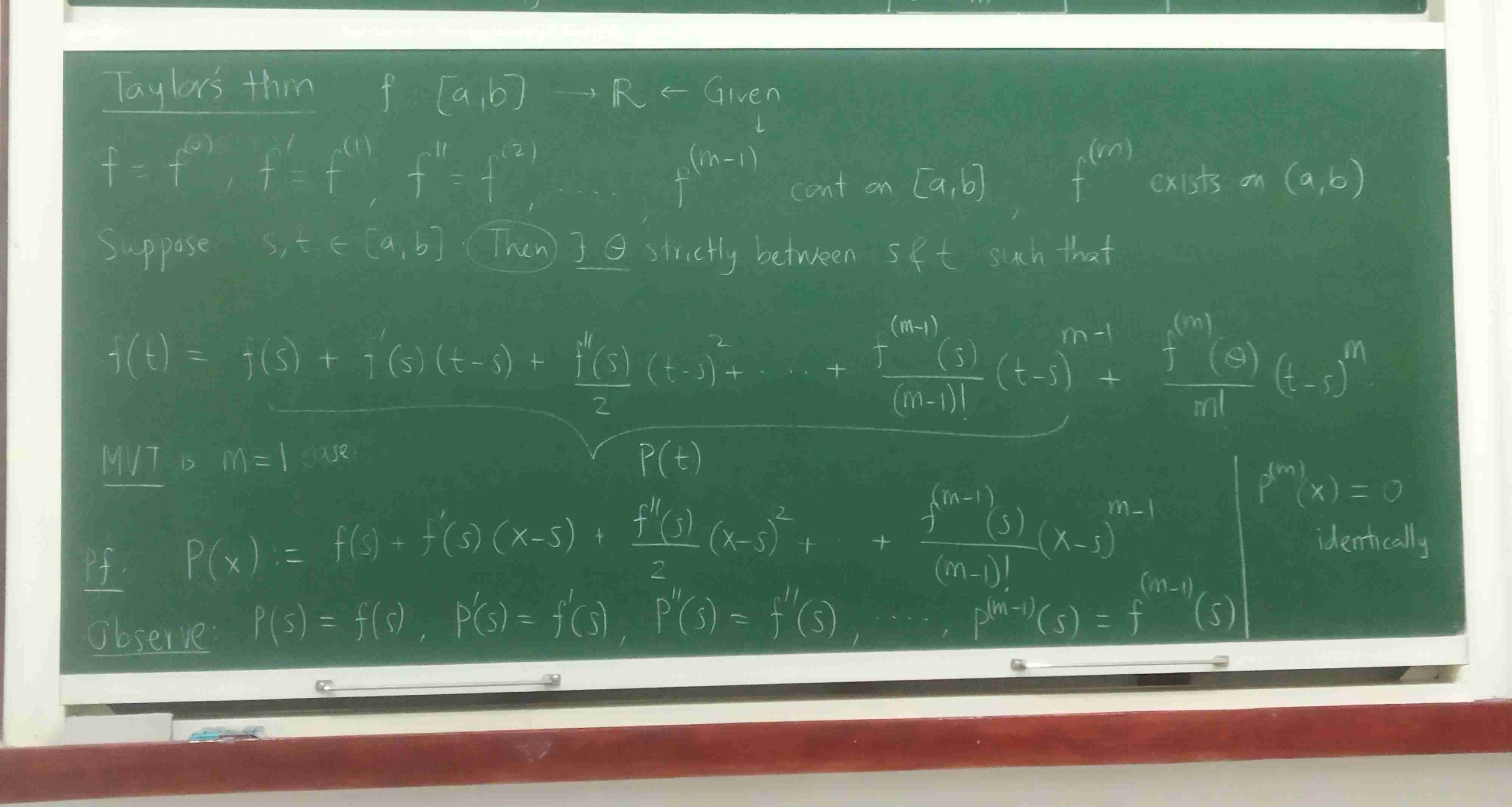
Theorem 147.3(Rudin 5.15).

Suppose $f:[a,b]\to \mathbb{R}$, and $f^{(0)},f^{(1)},\dots ,f^{(m-1)}$ are continuous on $[a,b]$, and $f^{(m)}$ exists on $(a,b)$. Let $x,x+h\in [a,b]$.
Then, there exists $\theta$ strictly between $x$ and $x+h$ such that

$$f(x+h)=\underset{E_{m-1}(h)}{\underbrace{f^{(0)}(x)+f^{(1)}(x)(h)+\frac{f^{(2)}(x)}{2}(h{)}^2+\cdots +\frac{f^{(m-1)}(x)}{(m-1)!}(h{)}^{m-1}}}+\frac{f^{(m)}(\theta )}{m!}(h{)}^m.$$

Proof.

We have shown that$f$ can be expressed as

$$f(x+h)=E_{m-1}(h)+r_{m-1}(h)h^{m-1}.$$

Let $M$ be the number defined by

$$f(x+h)=E_{m-1}(h)+M{h}^m.$$

Define

$$g(x+k)\equiv r_{m-1}(k)k^{m-1}-M{k}^m,$$

where $x+k\in [a,b]$. Note that $g(x)=0$, and $g(x+h)=0$. Also note that $g^{(1)}(x),g^{(2)}(x),\dots ,g^{(m-1)}(x)$ are zero.

On differentiating both sides $m$ times with respect to $k$ we get

$$g^{(m)}(x+k)=f^{(m)}(x+k)-Mm!$$

Now, since $g(x)=0$ and $g(x+h)=0$, there must exist $x+t_1$ between $x$ and $x+h$ such that $g^{\prime }(x+t_1)=0$, thanks to the mean value theorem. Again, since $g^{\prime }(x)=0$ and $g^{\prime }(x+t_1)=0$, there must exist $x+t_2$ between $x$ and $x+t_1$ such that $g^{\prime \prime }(x+t_2)=0$. After $m$ steps, we obtain $x+t_m\in (x,x+h)$ such that $g^{(m)}(x+t_m)=0$. Therefore, $M=\frac{f^{(m)}(x+t_m)}{m!}$.□

If we know that bounds on $|f^{(m)}(x)|$, we can bound the error!

---

MVT analogue for vector valued functions

The mean value theorem and L’Hospital’s rule are not true for complex or vector valued functions. For an example of the former, consider the map

$$\mathbf{f}:\mathbb{R}\to {\mathbb{R}}^2,\mathbf{f}(x)=(\cos x,\sin x).$$

${\mathbf{f}}^{\prime }(x)=(-\sin x,\cos x)$. Note that $|{\mathbf{f}}^{\prime }(x)|=1$ for all $x$. Now,

$$\begin{array}{r}\frac{\mathbf{f}(2\pi )-\mathbf{f}(0)}{2\pi }=0\ne {\mathbf{f}}^{\prime }(x)\forall x.\end{array}$$

However, an analogue of the MVT does exist:

Theorem 147.4(Rudin 5.19).

Suppose $\mathbf{f}$ is a continuous mapping of $[a,b]$ into ${\mathbb{R}}^k$ and $\mathbf{f}$ is differentiable in $(a,b)$. Then there exists $x\in (a,b)$ such that

$$|\mathbf{f}(b)-\mathbf{f}(a)|\le (b-a)|{\mathbf{f}}^{\prime }(x)|.$$

Proof.

Let$\mathbf{z}=\mathbf{f}(a)-\mathbf{f}(b)$. Define

$$\varphi (t)=\mathbf{z}\cdot \mathbf{f}(t).$$

Now, $\varphi$ is a continuous real function. Thus, the mean value theorem tells us

$$\varphi (a)-\varphi (b)=(b-a){\varphi }^{\prime }(x)=(b-a)\mathbf{z}\cdot {\mathbf{f}}^{\prime }(x)$$

for some $x\in (a,b)$. Also,

$$\varphi (b)-\varphi (a)=\mathbf{z}\cdot \mathbf{z}=|\mathbf{z}{|}^2.$$

Thus,

$$|\mathbf{z}{|}^2=(b-a)\mathbf{z}\cdot {\mathbf{f}}^{\prime }(x)\le (b-a)|\mathbf{z}||{\mathbf{f}}^{\prime }(x)|.$$ □

---

References

Pugh, C. C. (2015). Real Mathematical Analysis (2nd ed.). Springer International Publishing. https://doi.org/10.1007/978-3-319-17771-7