CM1 HW3

4.22

Part (a)

The $F=ma$ equations are

$$\begin{array}{rl}-mg-ky& =m\ddot{y}\\ -kx& =m\ddot{x}\end{array}$$

In the $y$ and $x$ directions respectively.

$$\begin{array}{r}\ddot{y}=-\left(g+\frac{ky}{m}\right)\end{array}$$

Let $w=g+\frac{ky}{m}$. Then, $\ddot{w}=\frac{k\ddot{y}}{m}$. Thus,

$$\begin{array}{r}\ddot{w}=-{\omega }^{2}w\end{array}$$

where ${\omega }^2=\frac{k}{m}$. This is a standard differential equation. Since we are given the initial position and velocity, it is beneficial to write the solution in this form:

$$\begin{array}{rl}w& =A\cos (\omega t)+B\sin (\omega t)\\ ⟹y& =A^{\prime }\cos (\omega t)+B^{\prime }\sin (\omega t)-\frac{gm}{k}.\end{array}$$

Plugging in the initial conditions of $y(0)=0$ and $\dot{y}(0)=v_0\sin \theta$, we get

$$\begin{array}{rl}{A}^{\prime }& =\frac{gm}{k},\\ B^{\prime }& =\frac{v_0\sin \theta }{\omega }.\\ & \\ \therefore y(t)& =\frac{gm}{k}\cos (\omega t)+\left(\frac{v_0\sin \theta }{\omega }\right)\sin (\omega t)-\frac{gm}{k}.\end{array}$$

Similarly, in the $x$ direction, we have

$$\begin{array}{r}x=C\cos (\omega t)+D\sin (\omega t).\end{array}$$

Plugging in the initial conditions of $x(0)=0$ and $\dot{x}(0)=v_0\cos \theta$, we get

$$\begin{array}{rl}C& =0,\\ D& =\frac{v_0\cos \theta }{\omega }.\\ & \\ \therefore x(t)& =\frac{v_0\cos \theta }{\omega }\sin (\omega t).\end{array}$$

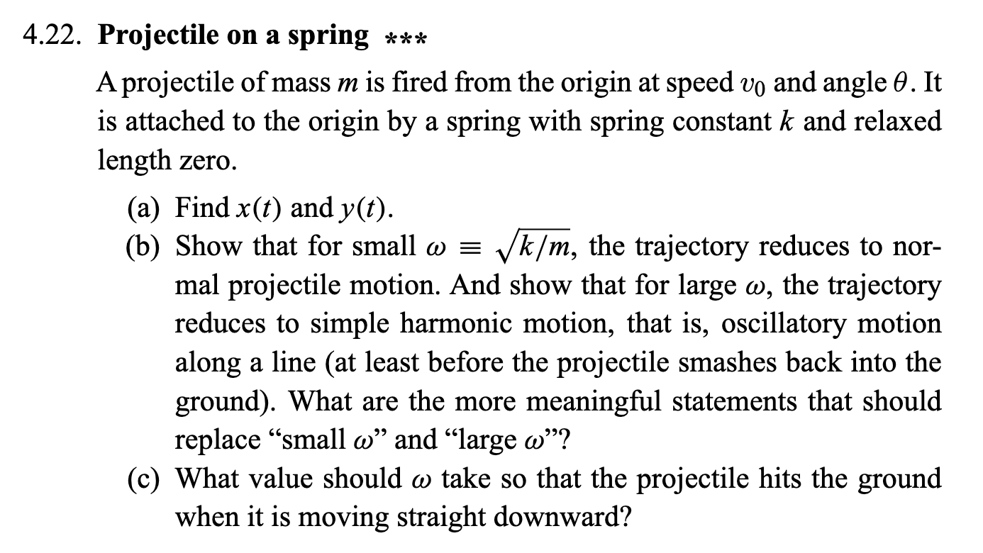
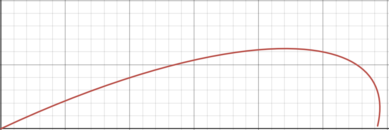
The trajectory looks elliptical:

---

Part (b)

If $\omega t\ll 1$, we can use the small angle approximations, namely $\sin \alpha \approx \alpha$ and $\cos \alpha \approx 1-\frac{{\alpha }^2}{2}$.

$$\begin{array}{rl}y(t)& \approx \frac{gm}{k}\left(1-\frac{{\omega }^2{t}^2}{2}\right)+\left(\frac{v_0\sin \theta }{\omega }\right)\omega t-\frac{gm}{k}=v_0\sin \theta t-\frac{1}{2}g{t}^2\\ x(t)& \approx \frac{v_0\cos \theta }{\omega }(\omega t)=v_0\cos \theta t\end{array}$$

These equations describe vanilla projectile motion. As stated initially, these approximations are only valid when $\omega t\ll 1$. If only we concern ourselves with the motion of the particle when it is airborne, $t$ attains its maximum value right before the particle hits the ground, which is $t=\frac{2v_0\sin \theta }{g}$. Thus, if $\omega \left(\frac{2v_0\sin \theta }{g}\right)\ll 1$, it follows that $\omega t\ll 1$ for all values of $t$ (before the particle hits the ground, of course). So, $\omega \ll \frac{g}{2v_0\sin \theta }$ would ensure that the small angle approximations are valid.

---

We notice that $y(t)$ can be rewritten like so:

$$y(t)=\frac{g}{{\omega }^2}(\cos (\omega t)-1)+\left(\frac{v_0\sin \theta }{\omega }\right)\sin (\omega t).$$

If we somehow get the first term to vanish, the trajectory is reduced to a straight line with slope $\tan \theta$.

$$\begin{array}{rl}y(t)& =\left(\frac{v_0\sin \theta }{\omega }\right)\sin (\omega t),\\ x(t)& =\left(\frac{v_0\cos \theta }{\omega }\right)\sin (\omega t).\\ & \\ ⟹& \frac{y}{x}=\tan \theta \end{array}$$

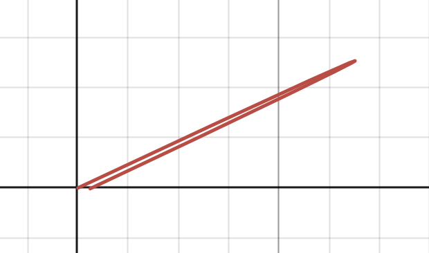
For this to happen, the first term must become negligibly small as compared to the second term. So,

$$\begin{array}{r}\frac{g}{{\omega }^2}\ll \frac{v_0\sin \theta }{\omega }\\ ⟹\omega \gg \frac{g}{v_0\sin \theta }\end{array}$$

---

Part (c)

We want $y=0$ when $\dot{x}=0$.

$$\begin{array}{r}\dot{x}=v_0\cos \theta \cos (\omega t)=0⟹\omega t=\frac{\pi }{2}\end{array}$$

Plugging $\omega t=\frac{\pi }{2}$ into $y(t)$, we get

$$\begin{array}{r}\frac{v_0\sin \theta }{\omega }=\frac{gm}{k}=\frac{g}{{\omega }^2}\\ ⟹\omega =\frac{g}{v_0\sin \theta }.\end{array}$$

---

4.29

$R$ is defined in 4.33 like so:

$$R\equiv \sqrt{{\left({\omega }^2-{\omega }_{\mathrm{d}}^2\right)}^2+(2\gamma {\omega }_{\mathrm{d}}{)}^2}.$$

On taking the derivatives of the expression inside the square root with respect to ${\omega }_d$, we get

$$\begin{array}{rl}& \frac{d}{d{\omega }_d}{R}^2=-4{\omega }_d({\omega }^2-{\omega }_d^2)+8{\gamma }^2{\omega }_d=4{\omega }_d^3+{\omega }_d(8{\gamma }^2-4{\omega }^2),\\ & \\ & \frac{d^2}{d{\omega }_d^2}{R}^2=12{\omega }_d^2+8{\gamma }^2-4{\omega }^2\end{array}$$

On setting the first derivative of $R^2$ equal to $0$,

$$\begin{array}{r}{\omega }_d\left({\omega }_d^2-({\omega }^2-2{\gamma }^2)\right)=0\end{array}$$

we get the critical points to be ${\omega }_{d_1}=0$ and ${\omega }_{d_2}=\sqrt{{\omega }^2-2{\gamma }^2}$.

On evaluating the second derivative at these points, we get $4(2{\gamma }^2-{\omega }^2)$ and $8({\omega }^2-2{\gamma }^2)$ respectively. Thus, if ${\omega }^2-2{\gamma }^2<0$, $R$ achieves a minima at ${\omega }_{d_1}$. If ${\omega }^2-2{\gamma }^2>0$, $R$ achieves a minima at ${\omega }_{d_2}$.

If ${\omega }^2-2{\gamma }^2=0$, we continue to take derivatives till we reach a non zero derivative:

$$\begin{array}{rl}& \frac{d^3}{d{\omega }_d^3}{R}^2=24{\omega }_d^{}\\ & \frac{d^4}{d{\omega }_d^4}{R}^2=24.\end{array}$$

Since $4$ is even and $24$ is positive, we can conclude from the higher order derivative test that ${\omega }_d=0$ is a minima.