AS DQN 1

Problem 1.4

For uncoupled systems of the form $\dot{\mathbf{x}}=A\mathbf{x}$ where $A=\text{diag}\{{\lambda }_1,\dots ,{\lambda }_n\}$, the solution is obtained by solving each of the uncoupled equations separately:

$$\mathbf{x}(t)=\left[\begin{array}{ccc}{e}^{{\lambda }_{1}t}& \dots & 0\\ ⋮& \ddots & ⋮\\ 0& \dots & e^{{\lambda }_{n}t}\end{array}\right]\mathbf{c}.$$

Therefore, $\mathbf{x}(t)\to 0$ as $t\to \infty$ for all $\mathbf{c}\in {\mathbb{R}}^n$ when ${\lambda }_i<0$ for all $i$.

This solution is unique, since the solution $x_i(t)=e^{{\lambda }_{i}t}{c}_i$ is unique for each equation in the system ($\frac{d}{dt}(x_i(t)e^{{\lambda }_{i}t})$ is constant).

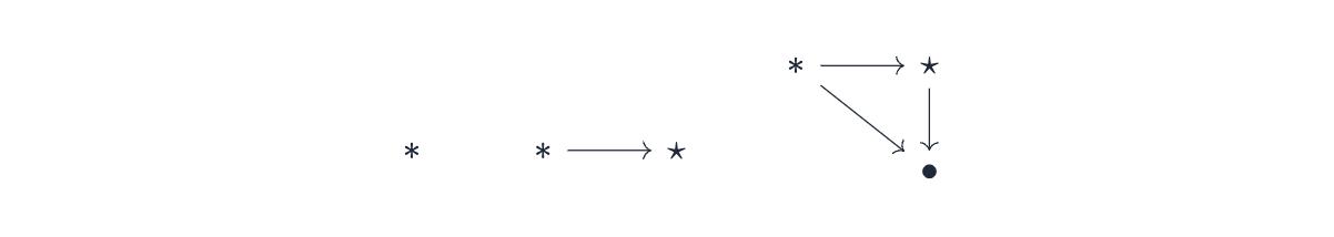
Problem 1.1

Part a

$$\begin{array}{r}\mathbf{x}(t)=\left[\begin{array}{cc}{e}^t& 0\\ 0& e^t\end{array}\right]\left[\begin{array}{c}{c}_1\\ c_2\end{array}\right].\end{array}$$ $$x_2=\frac{c_2}{c_1}{x}_1$$

Part b

$$\begin{array}{r}\mathbf{x}(t)=\left[\begin{array}{cc}{e}^t& 0\\ 0& e^{2t}\end{array}\right]\left[\begin{array}{c}{c}_1\\ c_2\end{array}\right].\end{array}$$ $$x_2=\frac{c_2}{c_1^2}{x}_1^2$$

Part c

$$\begin{array}{r}\mathbf{x}(t)=\left[\begin{array}{cc}{e}^t& 0\\ 0& e^{3t}\end{array}\right]\left[\begin{array}{c}{c}_1\\ c_2\end{array}\right].\end{array}$$ $$x_2=\frac{c_2}{c_1^3}{x}_1^3$$

Part d

The system yields the differential equation ${\ddot{x}}_1=-x_1$. Using an exponential ansatz of $x_1(t)=A{e}^{\alpha t}$, we see that $\alpha =\pm i$. Thus, a general solution has the form

$$x_1(t)=A{e}^{it}+B{e}^{-it}.$$

For the solution to be real, $A$ and $B$ are forced to be conjugates. Let $A,B=c_1\pm i{c}_2$. Then,

$$\begin{array}{rl}{x}_1(t)& =2c_1\cos t-2c_2\sin t\\ & =c_1\cos t+c_2\sin t,\end{array}$$

where $2c_1$ and $-2c_2$ have been renamed $c_1$ and $c_2$.

It follows that

$$x_2(t)=-{\dot{x}}_1=c_1\sin t-c_2\cos t.$$

Note that $x_1^2+x_2^2=c_1^2+c_2^2$ is constant for a given solution curve, making it a circle.

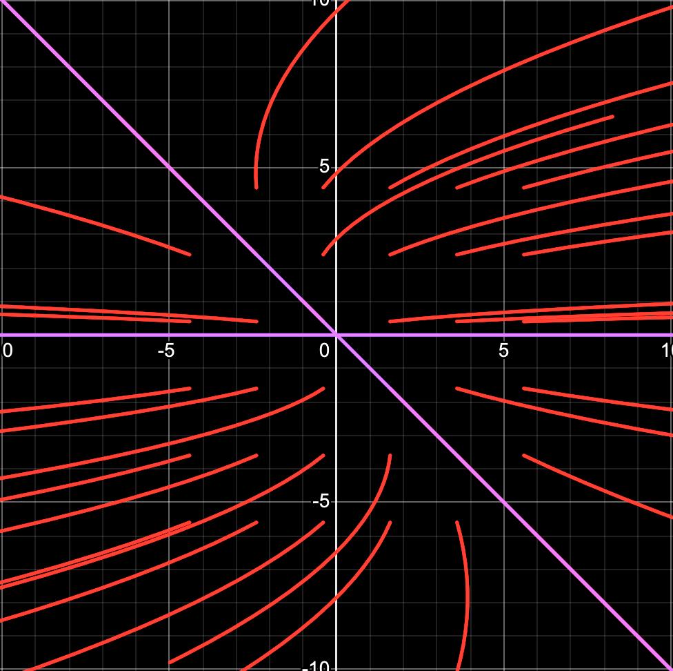
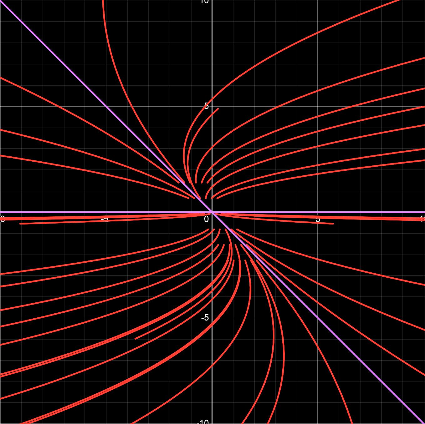
Part e

On finding $x_2(t)=c_2{e}^{-t}$, we obtain a first order linear differential equation

$${\dot{x}}_1+x_1-c_2{e}^{-t}=0$$

Applying the standard formula, we have $A(t)={\int }_0^{t}1dt=t$ and

$$\begin{array}{rl}{x}_1(t)& =c_1{e}^{-A(t)}+e^{-A(t)}{\int }_0^t{c}_2{e}^{-t}{e}^{A(t)}dt\\ & =c_1{e}^{-t}+e^{-t}{\int }_0^t{c}_{2}dt\\ & =c_1{e}^{-t}+c_{2}t{e}^{-t}.\end{array}$$

For $c_2>0$,

$$\frac{x_1}{x_2}+\ln x_2=\frac{c_1}{c_2}+\ln c_2$$

is constant for a given solution curve. For $c_2<0$,

$$\frac{x_1}{x_2}+\ln (-x_2)=\frac{c_1}{c_2}+\ln (-c_2)$$

is constant. For $c_2=0$, the solution is parameterized by $(c_1{e}^{-t},0)$.

---

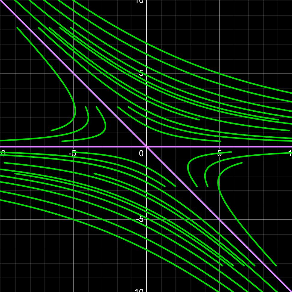
Problem 1.2

Part a

$$\begin{array}{r}\mathbf{x}(t)=\left[\begin{array}{ccc}{e}^t& 0& 0\\ 0& e^t& 0\\ 0& 0& e^t\end{array}\right]\left[\begin{array}{c}{c}_1\\ c_2\\ c_3\end{array}\right].\end{array}$$

Part b

$$\begin{array}{r}\mathbf{x}(t)=\left[\begin{array}{ccc}{e}^{-t}& 0& 0\\ 0& e^{-t}& 0\\ 0& 0& e^t\end{array}\right]\left[\begin{array}{c}{c}_1\\ c_2\\ c_3\end{array}\right].\end{array}$$

The $x_1,x_2$ plane is the stable subspace. The $x_3$ axis is the unstable subspace.

Part c

Observe that $x_1,x_2$ are uncoupled form $x_3$. Using previous work from Problem 1.1, part d, we have

$$\begin{array}{rl}{x}_1(t)& =c_1\cos t+c_2\sin t,\\ x_2(t)& =c_1\sin t-c_2\cos t,\\ x_3(t)& =c_3{e}^{-t}\end{array}$$

Clearly, the $x_3$ axis is the stable subspace.

---

Problem 2.6

Let ${\lambda }_1,\dots ,{\lambda }_n$ be the real, distinct eigenvalues of $A$, with corresponding eigenvectors ${\mathbf{v}}_1,\dots ,{\mathbf{v}}_n$. Then, $\dot{\mathbf{x}}=A\mathbf{x}$ has the solution

$$\mathbf{x}(t)=PE(t)P^{-1}\mathbf{x}(0),$$

where $P=\left[\begin{array}{ccc}{\mathbf{v}}_1& \dots & {\mathbf{v}}_n\end{array}\right]$ and $E(t)=\text{diag}(e^{{\lambda }_{1}t},\dots ,e^{{\lambda }_{n}t})$. Thus,

$$\varphi (t,{\mathbf{x}}_0)=PE(t)P^{-1}{\mathbf{x}}_0.$$

For fixed $t$, $\varphi (t,{\mathbf{x}}_0)$ is a linear map between finite dimensional vector spaces, and hence is continuous.

---

Problem 2.7

Part a

Let $\lambda =1$, $\mu =2$. We have

$$\begin{array}{rl}\mathbf{x}(t)& =\left[\begin{array}{cc}1& -1\\ 0& 1\end{array}\right]\left[\begin{array}{cc}{e}^t& 0\\ 0& e^{2t}\end{array}\right]\left[\begin{array}{cc}1& 1\\ 0& 1\end{array}\right]\mathbf{x}(0)\\ & =\left[\begin{array}{cc}{e}^t& e^t-e^{2t}\\ 0& e^{2t}\end{array}\right]\mathbf{x}(0)\end{array}$$

Part b

Let $\lambda =2$, $\mu =1$.

$$\begin{array}{rl}\mathbf{x}(t)& =\left[\begin{array}{cc}1& -1\\ 0& 1\end{array}\right]\left[\begin{array}{cc}{e}^{2t}& 0\\ 0& e^t\end{array}\right]\left[\begin{array}{cc}1& 1\\ 0& 1\end{array}\right]\mathbf{x}(0)\\ & =\left[\begin{array}{cc}{e}^{2t}& e^{2t}-e^t\\ 0& e^t\end{array}\right]\mathbf{x}(0)\end{array}$$

Part c

Let $\lambda =-2$, $\mu =-1$.

$$\begin{array}{rl}\mathbf{x}(t)& =\left[\begin{array}{cc}1& -1\\ 0& 1\end{array}\right]\left[\begin{array}{cc}{e}^{-2t}& 0\\ 0& e^{-t}\end{array}\right]\left[\begin{array}{cc}1& 1\\ 0& 1\end{array}\right]\mathbf{x}(0)\\ & =\left[\begin{array}{cc}{e}^{-2t}& e^{-2t}-e^{-t}\\ 0& e^{-t}\end{array}\right]\mathbf{x}(0)\end{array}$$

Part d

Let $\lambda =-1$, $\mu =1$.

$$\begin{array}{rl}\mathbf{x}(t)& =\left[\begin{array}{cc}1& -1\\ 0& 1\end{array}\right]\left[\begin{array}{cc}{e}^{-t}& 0\\ 0& e^t\end{array}\right]\left[\begin{array}{cc}1& 1\\ 0& 1\end{array}\right]\mathbf{x}(0)\\ & =\left[\begin{array}{cc}{e}^{-t}& e^{-t}-e^t\\ 0& e^t\end{array}\right]\mathbf{x}(0)\end{array}$$

Part e

Let $\lambda =1$, $\mu =-1$.

$$\begin{array}{rl}\mathbf{x}(t)& =\left[\begin{array}{cc}1& -1\\ 0& 1\end{array}\right]\left[\begin{array}{cc}{e}^t& 0\\ 0& e^{-t}\end{array}\right]\left[\begin{array}{cc}1& 1\\ 0& 1\end{array}\right]\mathbf{x}(0)\\ & =\left[\begin{array}{cc}{e}^t& e^t-e^{-t}\\ 0& e^{-t}\end{array}\right]\mathbf{x}(0)\end{array}$$

(lines are directed the opposite way!)

Part f

Let $\lambda =0$, $\mu =1$.

$$\begin{array}{rl}\mathbf{x}(t)& =\left[\begin{array}{cc}1& -1\\ 0& 1\end{array}\right]\left[\begin{array}{cc}1& 0\\ 0& e^t\end{array}\right]\left[\begin{array}{cc}1& 1\\ 0& 1\end{array}\right]\mathbf{x}(0)\\ & =\left[\begin{array}{cc}1& 1-e^t\\ 0& e^t\end{array}\right]\mathbf{x}(0)\end{array}$$

---

Problem 3.1

Part a

$\Vert A\Vert ={\max }_{|x|=1}|Ax|$. We need maximize $\sqrt{4x_1^2+9x_2^2}$ subject to the constraint $x_1^2+x_2^2=1$.

$$\begin{array}{rl}4x_1^2+9x_2^2& =4+5x_2^2,\end{array}$$

the maximum value of which is clearly $9$. Thus, $\Vert A\Vert =\sqrt{9}=3$.

Part b

We need to maximize $|Ax{|}^2=(x_1+2x_2{)}^2+x_2^2$ subject to the constraint $x_1^2+x_2^2=1$.

$$x_1^2+4x_1{x}_2+5x_2^2=1+4x_1{x}_2+4x_2^2.$$

Plug $x_1=\cos t$, $x_2=\sin t$, where $t\in [0,2\pi )$. We now need to maximize $f(t)=\sin t\cos t+{\sin }^{2}t$.

$$f^{\prime }(t)=\sin 2t+\cos 2t.$$

The zeroes of $f^{\prime }(t)$ are $3\pi /8,7\pi /8,11\pi /8,15\pi /8$. Of these, $t=3\pi /8$ and $t=11\pi /8$, correspond to local maxima, and the values of $f$ at these points are equal. Thus,

$$\begin{array}{rl}\Vert A\Vert & =\sqrt{1+4\cos \left(\frac{3\pi }{8}\right)\sin \left(\frac{3\pi }{8}\right)+4{\sin }^2\left(\frac{3\pi }{8}\right)}\\ & =1+\sqrt{2}.\end{array}$$

Part c

We need to maximize $|Ax{|}^2=26x_1^2+10x_1{x}_2+x_2^2$ subject to the constraint $x_1^2+x_2^2=1$. Again, let $x_1=\cos t$, and $x_2=\sin t$.

$$\begin{array}{rl}26x_1^2+10x_1{x}_2+x_2^2& =1+10x_1{x}_2+25x_1^2\\ & =1+10\cos t\sin t+25{\cos }^{2}t\end{array}$$

Let $f(t)=1+10\cos t\sin t+25{\cos }^{2}t$.

$$\begin{array}{rl}{f}^{\prime }(t)& =-10(2.5\sin 2t-\cos 2t)\end{array}$$

The zeroes of $f$ are

$$\left\{\left(\frac{k\pi +{\tan }^{-1}\left(\frac{2}{5}\right)}{2}\right):k\in \{0,1,2,3\}\right\}.$$

Of these, $k=0,2$ correspond to local maxima. Again, the values of $f$ at these points are equal. Thus,

$$\begin{array}{r}\Vert A\Vert =\sqrt{f\left(\frac{{\tan }^{-1}\left(\frac{2}{5}\right)}{2}\right)}=5.19258240357\dots .\end{array}$$